Determination of pressure loss along the length under uniform turbulent conditions. Darcy-Weisbach formula. Abstract: Coefficient of hydraulic friction

Formula for hydraulic resistance along the length of the pipeline

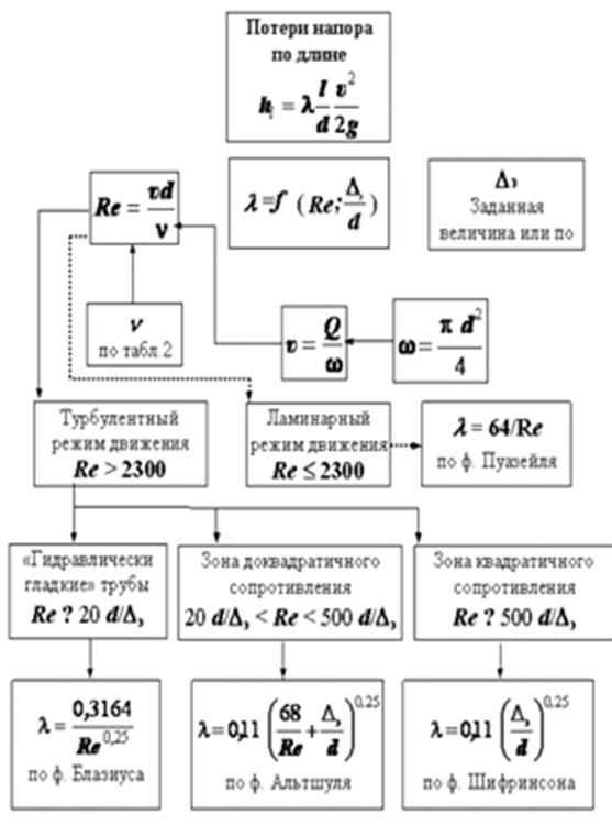
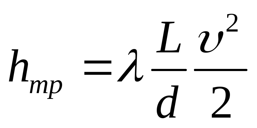
Pressure loss along the length of the pipeline is determined using the Darcy-Weisbach formula

Where – coefficient of hydraulic friction (Darcy coefficient). Losses significantly depend on the diameter of the pipes, the viscosity of the liquid, the speed of its movement and the roughness of the pipe walls. From the formula we can conclude that losses are proportional to the length of the pipe, inversely proportional to the diameter and proportional to the square average speed flow. However, such a conclusion will be valid only if the Darcy coefficient remains unchanged. In fact, the Darcy coefficient generally depends on the relative roughness of the pipeline walls and numbers Re, i.e.

.

Empirical study of pressure loss along the length of a pipe. Nikuradze's experiments

Coefficient determined experimentally (calculated using empirical formulas). Experimental data for in a wide range of Re numbers were obtained by Nikuradze. Artificial roughness was obtained by gluing sifted sand of a certain size to the inner surface of the pipe on a varnish base. Experiments were carried out for various liquids, roughness sizes and pipeline diameters. The experimental data obtained were summarized in Nikuradze’s graph and made it possible to reveal the mechanism of pressure loss along the length of the pipe. The graph shows the values of the hydraulic friction coefficient in logarithmic axes

from

at different values of relative roughness

. Here – absolute value of artificial roughness. The logarithm is used in order to cover the largest possible range of Re values, and at the same time, to represent in sufficient detail the region of small values of the Re number (laminar and transition modes of motion). Each fixed value on the graph corresponds to a separate curve, and the more , the higher the curve is.

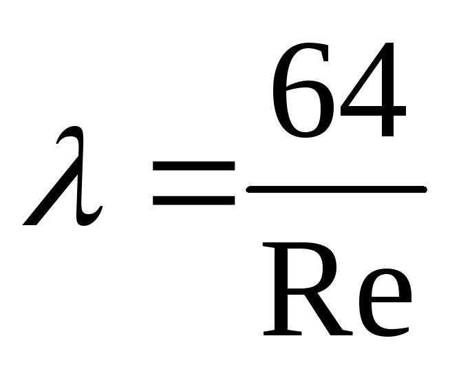
1. Laminar mode (on a straight line I). The Darcy coefficient does not depend on roughness. Expression for can be obtained theoretically

, it agrees well with experimental data.

2. Transitional mode (between straight lines I And II). It is usually assumed that the motion in this regime is turbulent (the laminar regime is unstable here) and the dependences of the turbulent regime are extrapolated to this region.

In the turbulent regime, three regions are distinguished.

3. Area of hydraulically smooth pipes (on a straight line II). In accordance with the previously considered structure of turbulent flow, the thickness of the viscous laminar layer at the wall

. The magnitude of all irregularities is less than the thickness of the laminar film. Here the Darcy coefficient does not depend on the roughness.

4. Pre-quadratic region (between straight lines II And III). The greater the roughness, the sooner the roughness protrusions leave the laminar wall film, and hence the exit from the region of hydraulically smooth pipes, i.e. the earlier the influence of roughness begins to appear.

5. Quadratic region (to the right of the line III). The Darcy coefficient does not depend on Re (“self-similarity” with respect to Re, i.e. independence from Re). The pressure loss along the length of the pipe is proportional to the square of the speed.

The Nikuradze graph allows us to explain the nature of hydraulic friction, however, since it was obtained for artificial roughness, it cannot be used for natural roughness. For real pipes, the emergence of roughness protrusions from the laminar wall film does not occur simultaneously, and the curves do not have a minimum.

For natural roughness, the concept of absolute equivalent roughness is introduced

, i.e. such a uniform roughness for which the losses in the quadratic mode are the same as for the natural roughness.

Formulas for determining the coefficient of hydraulic friction

1.

. Laminar mode.

. (The only case when the formula for the Darcy coefficient can be obtained theoretically. All other formulas are obtained from experimental data - empirical formulas). In a hydraulic drive course, the formula is usually used

, which takes into account losses in the initial section of the pipe (?).

2. . Transitional mode. As a rule, losses are calculated using formulas for turbulent mode (see below), however, for this area there is a rarely used Frenkel formula

.

3.

. Turbulent mode. Area of hydraulically smooth pipes. Blasius formula

. Sometimes found in the form

.

4.

. Turbulent mode. Pre-quadratic region.

Altschul's formula

. The most commonly used formula, recommended for use.

5.

. Turbulent mode. Quadratic resistance area.

Shifrinson's formula

.

Regions 4 and 5 are sometimes called the region of rough pipes (in contrast to region 3 - hydraulically smooth pipes), and region 5 is the region of completely rough pipes.

Altschul formula at large numbers Red coincides with the Shifrinson formula (the second term in brackets becomes negligibly small), and for small ones - with the Blasius formula (the first term is relatively small).

The Colebrook and White formula was experimentally obtained

check sound 27 min 10 lux

From (8.9) we can write the expression for the hydraulic slope

Then we have

Considering that the general expression for pressure loss along the length of pipes

equating it

Hence the Darcy coefficient

If we express the Re number in terms of the hydraulic radius R, then

The pressure loss along the length of a circular pipe with uniform laminar movement is proportional to the average flow velocity to the first power. This follows from (*), if we substitute , into this formula, and from (8.9b). Experimental data confirm the established dependence of h for on u to the first power.

To determine the pressure loss during laminar fluid flow in round pipe consider a section of pipe length l, along which the flow flows under laminar conditions (Fig. 4.3).

The pressure loss in the pipeline will be equal to

If in the formula the dynamic viscosity coefficient μ is replaced by the kinematic viscosity coefficient υ and density ρ (μ = υ ρ) and divide both sides of the equation by the volumetric weight of the liquid γ = ρ g, then we get:

Since the left side of the resulting equality is equal to the pressure loss h sweat in a pipe of constant diameter, then this equality will finally take the form:

The equation can be transformed into the universal Weisbach-Darcy formula, which is finally written as:

where λ is the coefficient of hydraulic friction, which for laminar flow is calculated by the expression:

However, in laminar mode, to determine the coefficient of hydraulic friction λ T.M. Bashta recommends for Re< 2300 применять формулу

This formula is called the Darcy-Weisbach formula and is one of

basic formulas of hydrodynamics.

The head loss coefficient along the length will be equal to:

Let's write the Darcy-Weisbach formula in the form:

The value is called the hydraulic slope, and the value is called

yut Chezy coefficient.

The quantity has the dimension of speed and is called dynamic

fluid speed.

Then the friction coefficient (Darcy coefficient):

Equivalent roughness- this is an artificial uniform roughness with such a height (diameter) of grains at which in the region of quadratic resistance (where it depends only on the roughness and does not depend on ) the value of the coefficient is equal to its value for natural roughness.

Hydraulically smooth and rough pipes. The condition of the pipe walls

significantly influences the behavior of a fluid in a turbulent flow. So when

laminar movement

the liquid moves slowly and smoothly, flowing calmly along its path

minor obstacles. The resulting local resistances

so insignificant that their magnitude can be neglected. In turbulent

in a flow, such small obstacles serve as a source of vortex motion of the fluid,

which leads to an increase in these small local hydraulic resistances,

which we neglected in laminar flow. With such small obstacles

the pipe wall is its irregularities. The absolute value of such irregularities

depends on the quality of pipe processing. In hydraulics, these irregularities are called

roughness protrusions, they are designated by the letter

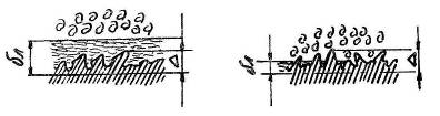
Depending on the ratio of the thickness of the laminar film and the size of the protrusions

roughness will change the nature of the fluid movement in the flow. When,

when the thickness of the laminar film is large compared to the size of the protrusions

roughness ( ,

roughness protrusions are immersed in the laminar film and turbulent core

they are inaccessible to currents (their presence does not affect the flow). Such pipes

are called hydraulically smooth (scheme 1 in the figure). When the size of the protrusions

roughness exceeds the thickness of the laminar film, then the film loses its

continuity, and roughness protrusions become the source of numerous

vortices, which significantly affects the fluid flow as a whole. Such pipes

are called hydraulically rough (or simply rough) (diagram 3 on

drawing). Naturally, there is an intermediate type of wall roughness

pipes, when the roughness protrusions become commensurate with the thickness

laminar film

(Scheme 2 in the figure). La thickness

minary film can be estimated based on the empirical equation

29. Determination of local resistance coefficients for sudden and smooth expansion, sudden and smooth narrowing, turning the pipe by

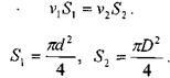
Then the amount of pressure loss during a sudden expansion of the channel will be determined:

Thus, we can say that the loss of head due to a sudden expansion of the flow is equal to the velocity head corresponding to the lost speed.

Smooth expansion of the channel (diffuser). The smooth expansion of the channel is called a diffuser. The fluid flow in the diffuser is complex. Since the live cross-section of the flow gradually increases, the speed of movement decreases accordingly fluid and pressure increases. Since, in this case, in the layers of liquid near the walls of the diffuser the kinetic energy is minimal (low speed), the liquid may stop and intensive vortex formation is possible. For this reason, the loss of pressure energy in the diffuser will depend on the loss of pressure due to friction and due to losses during expansion:

where: is the open cross-sectional area at the entrance to the diffuser,

S 2 - free cross-sectional area at the outlet of the diffuser, A - diffuser cone angle,

- correction factor depending on the conditions of flow expansion in the diffuser.

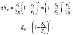
Sudden narrowing of the canal. With a sudden narrowing of the channel, the fluid flow breaks away from the walls of the inlet section and only then (in the section 2 - 2) touches the walls of the smaller channel. In this flow area - * two zones of intense vortex formation are formed (both in a wide section of the pipe and in a narrow one), resulting in, as in the previous case, pressure loss are made up of two components (friction losses and contraction losses). The coefficient of pressure loss due to the hydraulic resistance of a sudden narrowing of the flow can be determined from the empirical relationship proposed by I.E. Idelchikom:

Smooth narrowing of the channel. A smooth narrowing of the channel is achieved using a conical section called a confuser. Pressure losses in the confuser are formed almost due to friction, because There is practically no vortex formation in the confuser. The pressure loss coefficient in the confuser can be determined by the formula:

At a large taper angle A>50° the pressure loss coefficient can be determined by the formula with the introduction of a correction factor.

Rotate the channel. By such hydraulic resistance we mean the junction of pipelines of the same diameter, at which the axial lines of the pipelines do not coincide, i.e. make some angle between themselves A This angle is called the channel turning angle, because here the direction of fluid movement changes. The physical basis of the process of converting kinetic energy when turning the flow is quite complex and only the result of these processes should be considered. Thus, when passing through a section of sudden turn, a complex flow shape is formed with two zones of vortex fluid movement. In practice, such pipeline connection elements are called elbows. It should be noted that the elbow as a connecting element is extremely undesirable due to significant pressure losses in this type of connection. The value of the pressure loss coefficient will, first of all, depend on the angle of rotation of the channel and can be determined using an empirical formula or a table:

Laboratory work.

DETERMINATION OF THE HYDRAULIC FRICTION COEFFICIENT (DARCY COEFFICIENT).

1. Purpose of the work:

Studying methods for determining the coefficient of hydraulic friction;

Studying the methodology for experimental determination of the coefficient of hydraulic friction;

Establishing the dependence of the hydraulic friction coefficient on the Reynolds number.

2. Basic theoretical principles.

In real fluid flows, viscous friction forces are present. As a result, layers of liquid rub against each other as they move. This friction consumes part of the energy of the flow; for this reason, energy losses are inevitable during the movement. This energy, as with any friction, is converted into thermal energy. Because of these losses, the energy of the fluid flow along the length of the flow and in its direction is constantly decreasing, that is, the flow pressure H in the direction of movement the flow becomes less. If we consider two adjacent flow sections 1-1 and 2-2, then the loss of hydrodynamic head h will be:

Where H 1-1 - pressure in the first section of the fluid flow,

H 2-2 - pressure in the second section of the flow,

h- lost pressure - energy lost by each unit of weight of a moving fluid to overcome resistance along the flow path from section 1-1 to section 2-2.

Taking into account energy losses, the Bernoulli equation for the flow of a real fluid will look like

. (1)

Indices 1 and 2 indicate the flow characteristics in sections 1-1 and 2-2.

If we take into account that the characteristics of the flow - the average flow velocity  and the Coriolis coefficient  depend on the flow geometry, which for pressure flows is determined by the geometry of the pipeline, it is clear that energy (pressure) losses in different pipelines will vary differently.

There are two types of pressure losses - friction losses along the length of the pipeline and local losses.

Friction losses along the length.

When real (viscous) liquids flow through pipes and channels, pressure losses occur due to internal friction. These losses are proportional to the length of the channel section on which they occur, and are therefore called friction losses along the length.

Hydraulic losses in pressure flows occur due to a decrease in the specific potential energy of the liquid along the flow. In this case, the specific kinetic energy of the liquid, if it changes along the flow at a given flow rate, is not due to energy losses, but due to changes in the cross-sectional dimensions of the channel, since it depends only on the speed, and the speed is determined by the flow rate and cross-sectional area

In the general case, the magnitude of friction loss along the length is determined by the Darcy-Weisbach formula:

, (2)

Where  - average flow speed, L– length of the pipeline section, d– pipeline diameter,  - coefficient of hydraulic friction (Darcy coefficient).

Coefficient value  depends on the fluid flow regime.

In laminar flow mode  depends only on the Reynolds number and can be found by the formula:

. (3)

In turbulent conditions  in the general case, it is a function of both the Re number and the pipeline surface roughness (equivalent height of the roughness protrusions ). Specific type of addiction

depends on the ratio of roughness values and Re number. The most universal for turbulent flows is the Altschul formula:

. (4)

3. Description of the laboratory setup.

The hydraulic circuit diagram of the stand is shown in Figure 1.

The stand includes a hydraulic tank B, a gear pump H, a filter F, a safety valve KP, a flow regulator PP, two hydraulic valves P1 and P2, a spring accumulator A, two hydraulic throttles DR1 and DR2, and pipelines. The pump is driven by an electric motor. The information-measuring system of the stand includes 6 pressure gauges (MH1 - MH6, MH5 pressure gauge - electric contact with two controlled contacts), a high-speed flow meter RA, a thermometer T and an electronic stopwatch.

The hydraulic valves are controlled by toggle switches P1 and P2.

When setting the toggle switch to the “MANUAL” position an electronic stopwatch is used to determine the time it takes for a given volume of liquid to pass through the flow meter RA (in order to subsequently determine the liquid flow in the pipeline).

Rice. 1 Schematic diagram of the hydraulic stand

The power supply of the stopwatch is turned on with the “On” toggle switch, the time count starts with the “Counting” toggle switch, and the electronic scoreboard is reset with the “Reset” button. When you press the “Reset” button, the stopwatch should not count down time, that is, the “Count” toggle switch must be switched to the lower position.

The area studied in this work is the area ab.

4. Execution order:

4.1. Turn on the power of the stand;

4.2. Turn on the power to the electric motor;

4.3. Turn toggle switch P1 to the “On” position.

4.4. Allow the unit to operate for 5–6 minutes.

4.5. At different flow rates, record the pressures Pa and P b using pressure gauges МН1 and МН2, as well as the time of passage of a given volume of working fluid through the flow meter and the temperature of the liquid. Record the measurement results in a table in the test report.

4.6. After completing all experiments, turn off the power to the electronic stopwatch, electric motor and stand.

5. Processing of measurement results:

5.1. For each reading, using the Bernoulli equation (1), calculate the loss of pressure due to friction h tr .

, (5)

, (6)

where S is the cross-sectional area of the pipeline.

. (7),

where d is the internal diameter of the pipeline,  is the coefficient of kinematic viscosity of the liquid, which depends on the temperature according to Table 1.

Table 1. Kinematic viscosity coefficient of oil at various temperatures

5.3. Using the Darcy-Weisbach formula (2), knowing the amount of pressure loss h tr, express the coefficient of hydraulic friction for each experiment  .

5.4. Using formula (3) or (4) - depending on the observed flow regime - calculate the theoretical values of the coefficient of hydraulic friction   .

5.5. Enter the calculation results in Table 2.

table 2

			Re

5.6. Construct dependence graphs in one coordinate plane

And

.

The laboratory report must contain:

Test report

Laboratory work No. Determination of the coefficient of hydraulic friction.

Date of testing:

Performers:

Initial data:

Internal diameter of pipelines d= m

Length of the study area l= m

Oil density  = kg/m 3

Test results:

V, m 3	T, 0 C	P a , MPa	P b , MPa

Performers' signature

Teacher's signature

Abstract on the topic:

Darcy-Weisbach formula

Plan:

1 Darcy-Weisbach formula
2 Determination of the friction loss coefficient along the length
3 Determination of the Darcy coefficient for local resistances
4 History

Introduction

Weisbach formula in hydraulics - an empirical formula that determines head loss or pressure loss during developed turbulent flow of an incompressible fluid on hydraulic resistance (proposed by Julius Weisbach ( English) in 1855):

The Weisbach formula, which determines the pressure loss across hydraulic resistances, has the form:

Δ P- pressure loss across hydraulic resistance; ρ is the density of the liquid.

1. Darcy-Weisbach formula

If the hydraulic resistance is a section of pipe length L and diameter D, then the Darcy coefficient is determined as follows:

where λ is the friction loss coefficient along the length.

Then Darcy's formula takes the form:

or for pressure loss:

The last two dependencies are called Darcy-Weisbach formulas. Proposed by L. J. Weisbach (1845) and A. Darcy (1857).

If friction losses along the length are determined for a pipe of non-circular cross-section, then D represents the hydraulic diameter.

It should be noted that pressure losses on hydraulic resistances are not always proportional to the velocity pressure.

2. Determination of the friction loss coefficient along the length

The coefficient λ is determined differently for different cases.

For laminar flow in smooth pipes with rigid walls, the friction loss coefficient along the length is determined by the formula:

where Re is the Reynolds number.

Sometimes for flexible pipes the calculations take

For turbulent flow there are more complex dependencies. One of the most commonly used formulas is the Blasius formula:

This formula gives good results for Reynolds numbers varying from the critical Reynolds number Re cr to values Re = 10 5 . The Blasius formula is applied to hydraulically smooth pipes.

For hydraulically rough pipes, the friction loss coefficient along the length is determined graphically using empirical dependencies. Graphs for determining the friction loss coefficient along the length for rough pipes can be viewed here (k - roughness size, d - pipe diameter).

3. Determination of the Darcy coefficient for local resistances

Rice. 1. Hydraulic confuser: Q 1 - fluid flow in a wide section of the pipe; Q 2 - fluid flow in a narrow pipe section

For each type of local resistance there are its own dependencies for determining the coefficient ξ.

Some of the most common local resistances include sudden pipe expansion, sudden pipe contraction, and pipe rotation.

1. When sudden expansion pipes:

Where S 1 and S 2 - cross-sectional area of the pipe, respectively, before and after expansion.

2. When sudden contraction pipes, the Darcy coefficient is determined by the formula:

Rice. 2. Dependence of the Darcy coefficient on the angle δ of pipe rotation

Where S 1 and S 2 - cross-sectional area of the pipe, respectively, before and after the narrowing.

3. When gradual narrowing pipes (confuser):

where is the degree of narrowing; λ T- friction loss coefficient along the length in turbulent mode.

4. When sharp (without rounding) turn pipes (elbow), the Darcy coefficient is determined by graphical dependencies (Fig. 2).

4. History

Historically, the Darcy-Weisbach formula was obtained as a variant of the Prony formula.

Notes

Weisbach formula - www.femto.com.ua/articles/part_1/0437.html in the Physical Encyclopedia
Darcy-Weisbach formula - www.femto.com.ua/articles/part_1/0913.html in the Physical Encyclopedia

Literature

Hydraulics, hydraulic machines and hydraulic drives: Textbook for mechanical engineering universities / T. M. Bashta, S. S. Rudnev, B. B. Nekrasov and others - 2nd ed., revised. - M.: Mechanical Engineering, 1982.
Geyer V. G., Dulin V. S., Zarya A. N. Hydraulics and hydraulic drive: Textbook for universities. - 3rd ed., revised. and additional - M.: Nedra, 1991.

This abstract is based on

Determination of the coefficient of hydraulic friction

In the Bernoulli equation, written for two sections of a viscous fluid flow (standard notations):

where is the total amount of lost pressure:

where – pressure losses along the length of the design section of the pipeline, caused by friction of the liquid against the walls, are called path losses;

– pressure losses in short sections of the pipeline, caused by changes in shape or size (sometimes both at the same time), called losses in local resistance, or local pressure losses.

This paper examines travel losses. According to the continuity equation for the flow of a viscous incompressible fluid (ρ = const):

When fluid flows in a horizontal pipeline (z 1 =z 2) of constant cross-section (S 1 =S 2), the speed at the beginning and end of the calculated section will be the same (V 1 =V 2) and Bernoulli’s equation will take the form:

Travel losses are determined using the Darcy–Weisbach formula:

, (5)

where λ is the dimensionless coefficient of hydraulic friction (Darcy coefficient);

L – length of the design section of the pipeline;

d – pipeline diameter;

J – average flow speed.

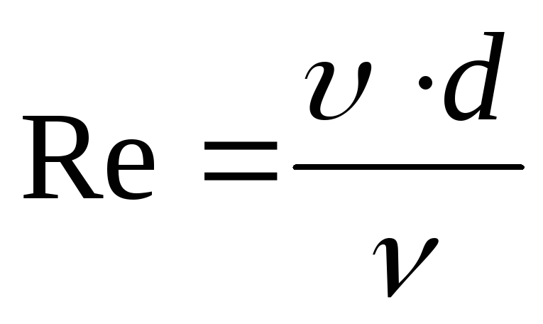
It has been experimentally established that the coefficient of hydraulic friction in the general case depends on the flow regime, characterized by the Reynolds number (Re), and the state of the inner surface of the pipeline, characterized by relative roughness (ε). The influence of these factors on the value of λ in laminar and turbulent flow regimes manifests itself differently.

In laminar mode, i.e. (ν is the kinematic viscosity coefficient), the state of the wall surface does not affect the resistance to fluid movement and λ = f (Re). The value of the coefficient λ in this case is determined by the theoretical Poiseuille formula:

Substituting this expression into (5), we obtain a formula for determining path losses in laminar flow in the form:

, (7)

From (7) it follows that in laminar flow, pressure losses along the length of the pipeline (path losses) are directly proportional to the average fluid flow velocity.

The turbulent flow regime is characterized by intense mixing of the liquid both in the transverse (along the cross-section of the flow) and longitudinal (along the length of the flow) directions. However, in the range of Reynolds numbers, immediately near the walls of the pipeline, there is a layer of moving fluid in which the flow remains laminar. This layer is called laminar sublayer or laminar film. The thickness of the laminar film (δ L) depends on the flow regime δ L = f (Re) and with increasing Reynolds number δ L decreases.

The walls of any duct have a natural surface roughness, initially determined by the material and manufacturing technology of the pipeline and changing during its operation due to the interaction of the pipeline material with the working fluid. The average height of the roughness protrusions (Δ) is called the absolute roughness. Depending on the relationship between δ L and Δ (see Fig. 1), pipes or walls are considered hydraulically smooth or hydraulically rough.

If δ L > Δ, the laminar sublayer seems to smooth out the wall roughness: the flow does not receive additional turbulization from the roughness, since the vortices formed at the tops of the roughness protrusions are suppressed by the laminar film. A pipe in which the roughness protrusions are within the thickness of the laminar sublayer is called hydraulically smooth.

If δ L< Δ, выступы шероховатости, оказавшись в турбулентном ядре потока, вносят дополнительное возмущение в обтекающую их жидкость, что приводит к увеличению сопротивления и, следовательно, потерь напора. Такая труба является гидравлически шероховатой.

Depending on the flow regime, the same pipe can be either hydraulically smooth or hydraulically rough, since with increasing Reynolds number the thickness of the laminar sublayer decreases, and, conversely, with increasing Re, δ L increases.

Natural roughness is always uneven, since the protrusions have different shapes, sizes and locations. Therefore, the concept of equivalent (or uniformly grained) absolute roughness Δ E is introduced. This artificially created roughness, for example, by gluing grains of sand of the same size (of the same fraction) and at equal distances from each other to the pipe walls, ensures the creation of pipeline resistance equal to the resistance at natural roughness.

The values of absolute (Δ) and equivalent (Δ E) roughness for pipes made of some materials are given in Table 1.

Table 1.

When determining λ, it is not the absolute roughness that is taken into account, but its relation to the diameter (or radius) of the pipe, i.e. relative roughness:

This is due to the fact that the same absolute roughness has a greater influence on the resistance to movement in a pipeline of smaller diameter.

A large number of empirical and semi-empirical formulas have been proposed for determining the coefficient of hydraulic friction λ, taking into account the features of flow in turbulent conditions. These features ultimately affect the dependence of travel losses on the average flow speed.

Thus, for hydraulically smooth pipes, the pressure loss along the length is proportional to the average speed to the power of 1.75. In the transition region from hydraulically smooth to rough pipes ( ) the value of λ is simultaneously influenced by two factors: the Reynolds number and the relative roughness, i.e. in the transition region λ = f (Re, ε). In this area, called the sub-square resistance zone, the pressure loss along the length is proportional to the average speed to the power of 1.74...2.

For hydraulically rough pipes, when the laminar film is almost completely destroyed, the coefficient λ no longer depends on Re, but is determined only by the relative roughness, i.e. λ = f(ε). This region is called a quadratic resistance zone, since hl ~J 2, or a self-similar region, since the independence of λ from Re means that the pressure loss along the length, determined by formula (5) is proportional to the square of the average speed. The beginning of this area is determined by the condition.

The most commonly used formulas for calculating the value of the coefficient λ are given in Table 2.

Determining λ using the formulas given in Table 2 and other formulas is facilitated by using tables and nomograms contained in educational and reference manuals.

When carrying out this work, flow regimes in hydraulically smooth pipes are considered.

table 2

Resistance zone, mode	Zone boundaries	Calculation formulas	Dependence of pressure loss on speed
1. Laminar		f. Poiseuille	h l ~J
2. Smooth-wall resistance zone		f. Blasius	h l ~J 1.75
2. Smooth-wall resistance zone		f. Konakova
3. Subquadratic resistance zone		f. Colebrook White	h l ~J 1.75 ¸ 2
3. Subquadratic resistance zone		f. Altshulya
4. Quadratic resistance zone		f. Prandtl-Nikuradze	h l ~J 2
4. Quadratic resistance zone		f. Shifrinson

Description of installation.

Schematic diagram experimental setup, used to determine the coefficient of hydraulic friction λ is shown in Fig. 2.

An experimental section of a circular pipeline of length L is connected to a pressure tank 5, into which water is continuously supplied from the water pipeline through valve 1 and a calming mesh 3. Excess water from the tank is drained through the overflow pipe 4. Therefore, a constant level in the tank can be maintained. The water flow through the experimental section is regulated by valve 7 (the valve at the entrance to the experimental section is completely open during the entire experiment). After passing through the experimental section, the water is drained into a measuring tank 8, at the inlet of which there is a tap 9. A thermometer 2 is installed to measure the water temperature. The installation is equipped with a piezometric shield 6, on which piezometers are installed to measure losses along the length.