When pumping oil through a main oil pipeline, the pressure developed by the pumps of pumping stations is spent on friction of the liquid against the pipe wall h , overcoming local resistance h ms, static resistance due to the difference in geodetic (leveling) marks z, as well as creating the required residual pressure in end of pipeline h stop .
The total pressure loss in the pipeline will be
H = h + h ms + z + h rest. (1.10)
pressure losses due to local resistances are 1…3% of linear losses. Then expression (1.10) takes the form
H = 1.02h + z + h rest. (1.11)
Residual head hres is necessary to overcome the resistance of technological communications and fill the tanks of the end point. The pressure loss due to friction in the pipeline is determined by the Darcy-Weisbach formula
or by the generalized Leibenson formula
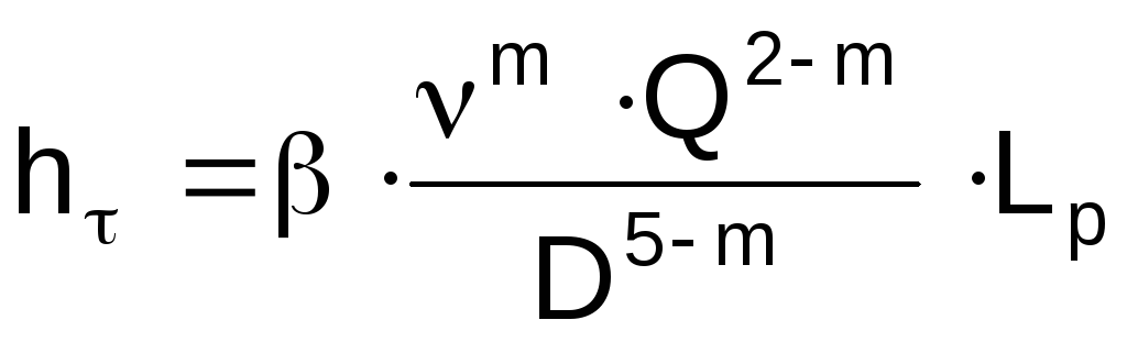 , (1.13)
where L p is the estimated length of the oil pipeline;
w - average speed oil flow through the pipeline;
– calculated kinematic viscosity of oil;
– coefficient of hydraulic resistance;
, m are the coefficients of the generalized Leibenson formula.
The values of , and m depend on the fluid flow regime and the roughness of the inner surface of the pipe. The fluid flow regime is characterized by the dimensionless Reynolds parameter
 , (1.14)
hydraulic slope
The hydraulic slope is called the loss of pressure due to friction, referred to the unit length of the pipeline
 (1.15)
Taking into account (1.15), equation (1.11) takes the form
9 Determination of the crossing point and the estimated length of the oil pipeline
Passing point called such a hill on the route of the oil pipeline, from which oil comes to the final point of the oil pipeline by gravity. In the general case, there may be several such vertices. The distance from the beginning of the oil pipeline to the nearest of them is called estimated length of the pipeline. Consider this using the example of an oil pipeline with a length L, a diameter D and a capacity Q
![]() .
.
From point a perpendicularly upwards, we set aside a segment ac equal to the value h l on the scale of heights.
Connecting the points b and c, we get the triangle abc, also called the hydraulic triangle. Its hypotenuse bc defines the position of the hydraulic slope line at the selected scale.
The point where line 2 touches the profile line indicates the position of the crossing point, which determines the estimated length of the pipeline.
This suggests that it is enough to pump oil to the transshipment point so that it reaches the final point of the pipeline with the same flow rate. Gravity of oil is ensured, since the available pressure (z PT - z K - h OT) is greater than the pressure required to overcome the resistance in the section from the crossing point to the final point
(z PT – z K – h OT)>i∙(L– l PT) ,
where l PT is the distance from the starting point of the oil pipeline to the transshipment point.
In this case, the distance L P \u003d l PT is taken as the estimated length of the pipeline, and the difference in geodetic marks is taken equal to z= z PT - z H. If there is no intersection of the hydraulic slope line with the profile, then the estimated length of the pipeline is equal to its total length L P =L, and z= z K - z H .
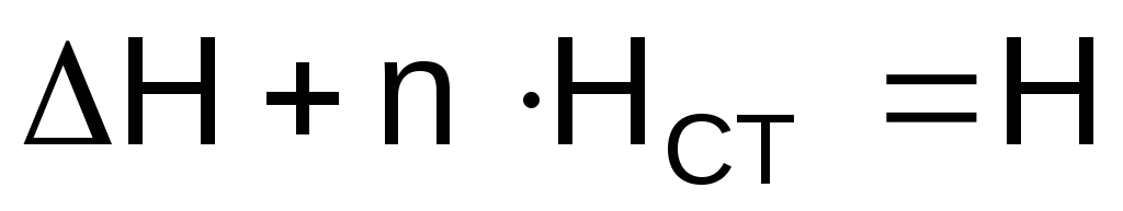
10. For a main oil pipeline of constant diameter with n pumping stations, balance equation pressure has the form .
At the beginning of each operational section, the substations are equipped with booster pumps. At the end of the pipeline and each production section, it is required to provide a residual head h OST to overcome the resistance of process pipelines and injection into tanks.
The right side of equation (1.34) is the total pressure loss in the pipeline, i.e. N. In the case of inserts or loopings along the route, the right side of equation (1.34) is determined by formula (1.32).
The left side of equation (1.34) is the total head developed by all operating pumps of pumping stations (active head). With the help of pump performance coefficients, the active total head can be represented by the dependence
a P, b P, h P - coefficients of performance and pressure developed by the booster pump when Q is supplied;
 And
And
 ,
(1.36)
,
(1.36)
Expressing the left side of equation (1.34) through (1.35), and the right side through (1.30), we obtain the pressure balance equation in analytical form
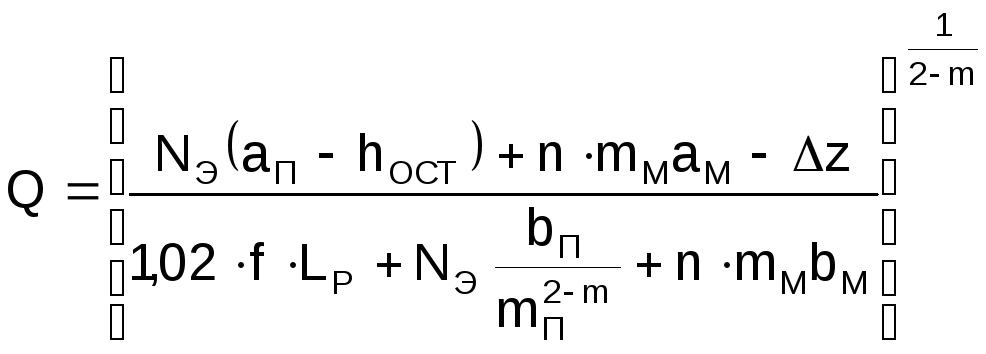 . (1.38)
If in the general case there are loopings and inserts on the linear part, equation (1.38) takes the form
 .
(1.39)
.
(1.39)
11 .The point of intersection of the characteristics is called the operating point (A), which characterizes the pressure loss in the pipeline and its capacity under given pumping conditions (Fig. 1.12). The equality of the generated and expended pressures, as well as the equality of the supply of pumps and the flow of oil in the pipeline, lead to an important conclusion: the pipeline and pumping stations make up a single hydraulic system. Changing the operating mode of the PS (shutdown of some pumps or stations) will lead to a change in the mode of the oil pipeline as a whole. Changes in the hydraulic resistance of a pipeline or its individual run (changes in viscosity, inclusion of reserve lines, replacement of pipes in certain sections of the route, etc.) will, in turn, affect the operation of all pumping stations.
(Lab #6)
GENERAL INFORMATION
In the hydraulic calculation of water pipelines, heat exchangers, technological systems of pumping stations, water collection and treatment systems, it is necessary to determine the loss of specific energy (energy per unit weight of the liquid). Losses of specific energy (pressure loss) are caused by the friction of the liquid against the pipeline walls, the friction that occurs between the moving layers of the liquid, as well as their mixing. As shown by theoretical studies, confirmed by experience, the pressure loss during the movement of fluid through the pipeline depends on the mode of movement of the fluid (Reynolds number Re), diameter, length of the pipeline, pipe roughness and fluid velocity. These losses are determined by the Darcy formula:
where l - Darcy coefficient(hydraulic resistance coefficient);
l is the length of the pipeline;
d is the inner diameter of the pipeline;
V is the average velocity of the liquid in the pipeline;
g is the free fall acceleration.
It is easy to see that to determine the pressure loss along the length, you need to know the value of l. In physical terms, l means what part of the velocity head (V 2 /2q) is the loss per unit relative length of the pipe (l / d).
With a uniform isothermal laminar flow of fluid in a pipe of circular cross section, the Darcy coefficient is determined by the theoretical Stokes formula
For the same conditions turbulent regime fluid flow, the Darcy coefficient is calculated using empirical and semi-empirical formulas obtained on the basis of theoretical and experimental studies. These studies have shown that with an increase in the Re number, the degree of its influence on l decreases, while the degree of influence of roughness increases. The physical explanation of such a phenomenon is based on the Prandtl hypothesis. In accordance with the above hypothesis, the turbulent flow can be conditionally divided into two areas (Fig. 4): a viscous sublayer (1) located at the inner wall of the pipe (2), and a turbulent core in its center (3).
The fluid flow in the viscous sublayer is formed under the influence of the interaction of external forces with the forces of viscosity. The flow in a turbulent core, according to Prandtl, occurs under the influence of the interaction of external forces with the friction force that appears due to mixing.
 Rice. 4
The thickness of the viscous sublayer δv depending on the speed of movement is calculated by the formula:
It can be seen from dependence (15) that the greater the fluid flow rate, the smaller (ceteris paribus) the thickness of the viscous sublayer. At low speeds (small Reynolds numbers), the thickness of the viscous sublayer increases. It becomes larger than the roughness protrusions of the inner machine tool of the pipe, and they do not affect the flow in the core and l.
At high speeds (large Reynolds numbers), the thickness of the viscous sublayer is small. Roughness protrusions not covered by a viscous sublayer have a direct effect on the flow in the core, determining the value of the coefficient l. Therefore, depending on the ratio of the roughness projections D and the thickness of the viscous sublayer δ in pipes, they are divided into hydraulically smooth (D< δ в) и гидравлически шероховатые (D >δ c). Taking into account formula (3), it can be argued that the same pipe can be both hydraulically smooth and hydraulically rough. This means that the coefficient l will be different for hydraulically smooth and rough pipes.
Experiments show that, depending on the ratio of D and δ at turbulent flow liquids, three laws of friction are observed. Each of them is valid only in a certain range of change in the Reynolds number.
In turbulent fluid flow, three friction zones are distinguished: smooth, mixed, and rough, determined by the ratio of the magnitude of the roughness protrusions and the pipe diameter. Since the resistance to fluid flow depends not only on the height of the protrusions, but also on their shape, relative position, the number of protrusions per unit area, and other factors, the concept of “equivalent” roughness (Ke), determined experimentally, is introduced.
The zone of smooth friction begins with the Reynolds number (3.5 - 4) × 10 3 and ends at its first boundary value (Re '), determined by the formula
where is the relative equivalent roughness equal to K e /d.
The Darcy coefficient in this friction zone is determined by the Blasius formula
 (17)
(17)
The mixed friction zone starts at the first Reynolds number Re' and ends at the second Re” = 500/ . In this friction zone, to determine the Darcy coefficient, you can use the formula of A.L. Altshulya
 . (18)
In the rough friction zone, the Reynolds numbers are greater than the second boundary value Re” > 500/ . In this zone, the value of 68/Re becomes negligible compared to , the Altshul formula turns into the Shifrinson formula
L = 0.11 × () 0.25 , (19)
valid for Re > Re” and £ 0.007.
If Re > Re” and > 0.007, the calculation of the Darcy coefficient is carried out according to the Prandtl-Nikuradze formula
 (20)
(20)
Since the Darcy coefficient in the rough friction zone is determined only by the relative equivalent roughness, formula (19, 20) also serves to find .
The equivalent roughness values are given in the reference literature on hydraulics. The tables of values are compiled on the basis of experimental data, taking into account the material, the method of manufacture and the condition of the pipes. The condition of the pipes takes into account: cleanliness, service life, the presence of corrosion.
Therefore, having data on the equivalent roughness of the pipeline walls and knowing its diameter, it is possible to determine the boundary conditions for Reynolds numbers and the friction zone.
In addition to the considered conditions of analytical methods for determining the Darcy coefficient, there are also graphical dependences l on Re and K e. For steel technical pipes these graphs are based on the results of experimental studies carried out in our country by Murin G.A.
For specific conditions, the coefficient can be determined empirically.
GOAL OF THE WORK
Mastering the experimental and calculation methods for determining the pressure loss due to friction along the length.
Consider kinds hydraulic resistance .
When a fluid moves, part of the pressure is spent on overcoming various resistances. Hydraulic losses depend mainly on the speed of movement, therefore the head is expressed in fractions of the velocity head
Where - coefficient of hydraulic resistance, showing what proportion of the velocity head will be the lost head,
or in pressure units:
Such an expression is convenient in that it includes a dimensionless proportionality factor, called the drag coefficient, and velocity head, which is included in the Bernoulli equation. The coefficient , thus, is the ratio of the lost head to the velocity head.
Head loss during fluid movement is caused by two types of resistance: length resistance, determined by friction forces, and local resistance, due to changes in flow velocity in direction and magnitude.
local losses energies are due to the so-called local resistances: local changes in the shape and size of the channel, causing deformation of the flow. When a liquid flows through local resistances, its velocity changes and vortices usually appear.
The following devices can serve as examples of local resistances: valve, diaphragm, elbow, valve, etc. (Fig. 37).
The head lost to overcome local resistances in linear units is determined by the formula:
(this expression is often called the Weisbach formula),
and in units of pressure:
where: - coefficient of local resistance, usually determined empirically (the values of the coefficient are given in reference books depending on the type and design of local resistance),
is the specific gravity of the liquid,
is the density of the liquid,
V- the average speed in the pipeline in which this local resistance is installed.
Gate valve Elbow Fork flow

 Valve Restriction Merging
 Diaphragm Expansion Valve with Mesh

Figure 37 - Examples of local hydraulic resistance
Figure 38 - Design speed selection.
If the diameter of the pipeline changes, therefore, the speed in it changes over a short section, then it is more convenient to take the larger of the speeds as the design speed in the calculation (Fig. 38). For example, a sudden narrowing of the pipeline, the entrance to the pipeline, etc. ( , the design speed is taken V = V 2).
Friction loss or linear resistances are caused by friction forces that occur along the entire length of the fluid flow at uniform motion, so they increase in proportion to the length of the stream. This type of loss is due to internal friction in the liquid, and therefore it occurs not only in rough, but also in smooth pipes.
The loss of pressure due to friction (along the length) can be determined by the formula:
However, it is more convenient to associate the coefficient with the relative length l/d. Let's take a plot round pipe length equal to its diameter d and denote the coefficient of its resistance, which is included in the formula through . Then for the entire pipe length L and diameter d coefficient will be l/d times more, namely:
where is the coefficient of hydraulic friction, or the Darcy coefficient,
L- section length,
d- pipe diameter.
Such a replacement allows us to bring the formula to a form that is very convenient for practical use:
The formula is usually called the Darcy-Weisbach formula. The friction coefficient λ in most cases is determined empirically depending on the Reynolds criterion Re and surface quality (roughness).
Head loss summation
In many cases, when fluids move in various hydraulic systems(for example, pipelines) there are simultaneous losses of pressure due to friction along the length and local losses. The total head loss in such cases is defined as arithmetic sum losses of all kinds.
When determining the losses in the entire flow, it is assumed that each resistance does not depend on the neighboring ones. Therefore, the total loss is the sum of the losses caused by each resistance.
If the pipeline consists of several sections with lengths of different diameters with several local resistances, then the total head loss is found by the formula:
 ,
,
Where ![]() ,
,
, ,…, , , , …, , , , …, are resistance coefficients and average speeds for individual sections and local resistances.
3.6 Influence of various factors on the ratio
The greatest difficulty in calculating pressure losses is the calculation of the coefficient of hydraulic friction , which is influenced by many flow and pipeline parameters.
The study of the influence of various factors on the value of the coefficient of hydraulic friction is devoted to big number experimental and theoretical works. These experiments were carried out most thoroughly by I. Nikuradze (1932). They were carried out on pipes with artificial roughness, which was created by gluing sand grains of uniform roughness to the inner surface of the pipes. The head loss in the pipes was determined at various flow rates, and the coefficient was calculated using the Darcy–Weisbach formula , whose values were plotted on a graph as a function of the Reynolds number Re.
The results of Nikuradze's experiments are presented in the graph = f(Re) (Fig. 39). Considering it, we can draw the following important conclusions.
In the region of the laminar regime ( Re<2320) все опытные точки независимо от шероховатости стенок уложились на одну прямую (линия 1).
Therefore, depends here only on the Reynolds number and does not depend on the roughness.
In the transition from laminar to turbulent regime, the coefficient increases rapidly with increasing Re, while remaining independent of roughness in the initial section.
Three zones of resistance can be distinguished in the region of the turbulent regime. The first is the zone of smooth pipes, in which = f(Re), and the roughness Ke() does not appear, in the figure the points are located along an inclined curve (curve 2). The deviation from this curve occurs the earlier, the greater the roughness.
The next zone is called the zone of rough pipes (pre-square), in the figure it is represented by a series of curves 3 tending to certain definite limits. The coefficient in this zone depends, as can be seen, both on the roughness and on the Reynolds number = f(Re, Ke/d). And, finally, when certain values of the numbers Re are exceeded, curves 3 turn into straight lines parallel to the axis Re, and the coefficient becomes constant for a constant relative roughness = (Ke/d). This zone is called self-similar or quadratic.
 Figure 39 – Nikuradze Charts
Approximate area boundaries are as follows:
smooth pipe zone 4000
rough pipe zone 10 d/Ke
quadratic zone Re> 500d/Ke.
The transition from one zone to another can be interpreted as follows: as long as the projections of the roughness are completely immersed in the laminar boundary layer (i.e.< ), они не создают различий в гидравлической шероховатости. Если же выступы шероховатостей выходят за пределы пограничного слоя (Ke>δ), the roughness projections come into contact with the turbulent core and vortices are formed. As is known, with increasing Re the layer thickness decreases and in the last zone (quadratic) this layer disappears almost completely ().
However, the pipes used in practice have non-uniform and non-uniform roughness. Many scientists were engaged in clarifying the issues of influence on natural roughness, the experiments of G. A. Murin (for steel pipes) received the greatest fame.
Confirming the basic regularities established by Nikuradze, these experiments made it possible to draw a number of important and essentially new conclusions. They showed that for pipes with natural roughness in the transition region it always turns out to be greater than in the quadratic region (and not less, as in the case of artificial roughness); and upon transition from zones 2–3 to the fourth, the continuity decreases. The results of Murin's experiments are shown in Figure 40.


![]()


Figure 40 - Results of Murin's experiments
3.7 Formulas for determining the Darcy coefficient
To calculate the Darcy coefficient, there are a very large number of empirical and semi-empirical formulas, most of which have a limited area of application. We will consider only a few basic, most commonly used formulas that have wide boundaries.
In laminar mode ( Re<2320) для определения в круглых трубах применяют формулу Пуазейля:
= 64/Re.
The formula was derived theoretically, which is shown in the section "Peculiarities of the flow in laminar regime".
In the region of transition from laminar to turbulent regime λ calculated by the Frenkel formula:
λ= 2,7/Re 0,53 .
In turbulent conditions, there are three zones:
For hydraulically smooth pipes, several formulas are used:
Most commonly used:
Blasius λ= 0,3164/Re 0.25 scope (4000<Re<10 5);
Konakova λ= 1/(1.81lg Re- 1.5) 2 scope (4000<Re<3×10 6)
For hydraulically rough pipes:
Altshulya λ= 0,11(K E /d+ 68/Re) 0,25 ;
Colebrook-White
The boundaries of the use of these formulas can be determined in the range of Reynolds numbers from 10 d/K E up to 500 d/K E.
In the region of quadratic resistance (Reynolds numbers over 500 d/K E) formulas are applied:
Shifrinson B. L. λ= 0,11(K E /d) 0,25 ;
Prandtla - Nikuradze λ= 1/(1,74+ 2lg d/K E) 2 .
The above formulas most fully and correctly take into account the influence of various factors on the coefficient of hydraulic friction. They are selected from a large number of formulas that currently exist.
A. D. Altshul's formula is the most universal and can be applied to any of the three zones of the turbulent regime. At low Reynolds numbers, it is very close to the Blasius formula, and at high Reynolds numbers, it is converted into the Shifrinson formula by B. L.
Control questions
1. Two modes of movement of liquids and gases.
2. Reynolds experiments, Reynolds criterion.
3. Features of laminar and turbulent regimes.
4. Velocity distribution diagrams.
5. Hydraulic resistance, their physical nature and classification.
6. Formulas for calculating energy losses (pressure).
7. Local hydraulic resistance, basic formula.
8. Dependence of the coefficient of local resistance on the Reynolds number and geometric parameters.
9. Resistance along the length, the main formula for calculating losses.
10. Hydraulic resistance zones, experiments by Nikuradze and Murina.
11. The most commonly used formulas for calculating the hydraulic coefficient of friction.